DeepMedic - multi-sacle 3D CNN with CRF for brain lesion segmentation
论文阅读笔记,如果我有什么理解错误的地方,欢迎大家指正。
论文:Efficient multi-scale 3D CNN with fully connected CRF for accurate brain lesion segmentation
摘要:作者提出一种双路径,11层深的3D卷积神经网络用于brain lesion segmentation任务,主要解决了医学图像处理上的三个方面的问题。一是作者设计了一种dense training scheme的方案,采用全卷积神经网络,一次把相邻像素的image segments传入网络输出dense prediction (dense-inference),从而节省了计算代价。作者使用更深的网络使模型判别能力更强。作者使用一种dual pathway architecture,即同时训练两个网络,使模型同时对高/低分辨率图像进行处理。最后作者采用全连接条件随机场(Fully connected Conditional Random Field)对网络output进行后处理(post-processing)改善图像类之间的边缘信息。
1. Dense Training
在传统patch-wise的分类中,输入patch的尺寸和cnn最后一层神经元的感受野大小相同,这样网络得到一个single prediction对应输入patch的中心像素的值。而用全卷积实现的神经网络,因为其输入的patch的尺寸可以大于最后一层神经元的感受野,因此模型可以同时输出多个prediction,即dense-inference,而每一个prediction对应cnn’s receptive field的在输入patch上的每一步stride。

同时作者认为,这样dense-inference得到的每一个prediction都是可信的,只要感受野是完全在input patch上扫过,并且只捕捉到原始信息,因此没有使用padding。
Dense Training Scheme 的优点
- 节省计算代价和内存消耗
- 灵活:作者提到最佳的性能为将整个图像送入网络,但是这个做法不现实。如果GPU内存限制不允许,例如在需要缓存大量FM的大型3D网络的情况下,则将图像分成多个image-segments,这样会比单个segment大,但是可以去fit内存。(原文:If GPU memory constraints do not allow it, such as in the case of large 3D networks where a large number of FMs need to be cached, the volume is tiled in multiple image-segments, which are larger than individual patches, but small enough to fit into memory.)
CNNs are trained patch-by-patch: 个人认为论文中提到的这个操作是在图像上randomly crop出一个individual patch作为网络的输入来训练网络,以此计算loss和进行gradient descent。
2. Class Balance
(这里不太确定自己理解对不对)
在原文的Section 2.2中作者提到,这种dense training scheme的方案中的sampling input segments (即上面提到的randomly crop individual patches) 提供了一种灵活的方式去平衡training samples中的segmentation classes(正负类)的分布,而不同的分布对模型的性能有很大的影响。
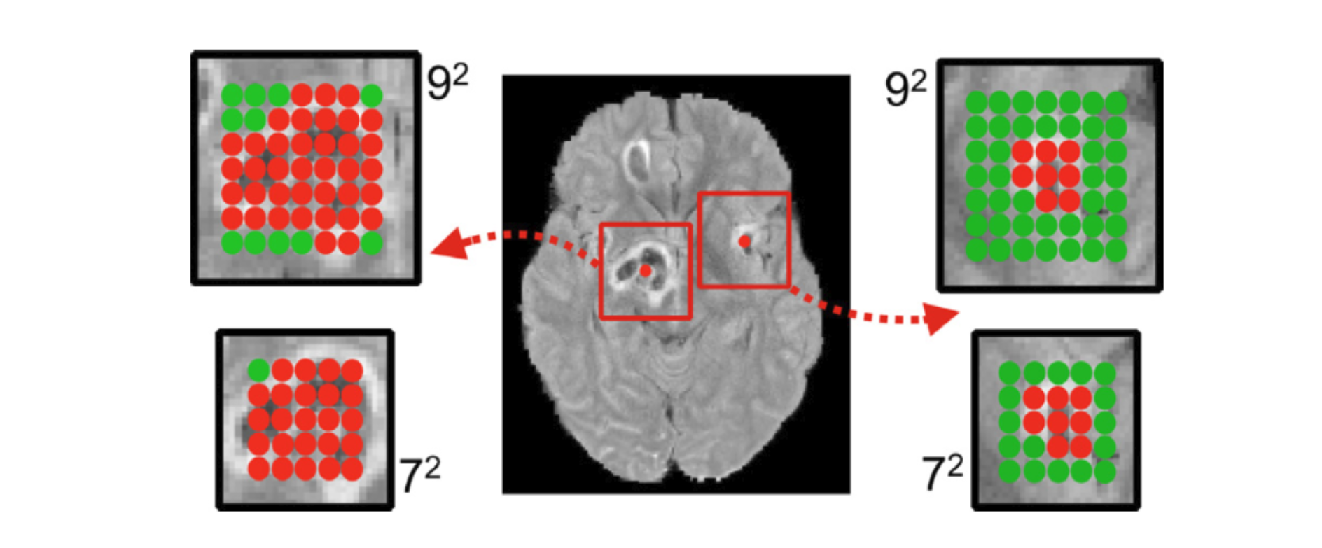
从上图和原文Section 3.2的实验结果来看,感觉有点类似过采样的意思。上图说明,如果是crop一个以病变为中心 (lesion-centered) 的image segments,分别用 $7 \times 7$ 和 $9 \times 9$ 的框去crop下来,可以看到用 $9 \times 9$ 的框去crop出这个image segment的话,绿色的内容会相对更多一点。
作者在Section 3.2的最后一段也提到,这个segments size在模型中是一个超参数,提到segment size会提升模型的性能,但是很快这种性能的提升久会达到平稳(level off),并且在一系列的segment size中都会得到相似的性能。
3. 构建更深的网络
该部分总结:Deeper Networks + Smaller Kernel + Batch Norm + (p)ReLU + $ \mathcal{N}\left(0,\ \sqrt{2/n^{in}_{l}} \right)$
更深的网络有更好的判别能力,但是更深的网络同时意味着更高的计算代价和更吃内存。所以在这里作者采用的策略是层数增加,但是把kernel size从 $5^3$ 缩小到 $3^3$ 从而减少计算代价和节省内存。作者认为这里kernel size减小说明需要训练的parameters的数量减少,一定程度上有正则的效果。(但是原文好像只是给了个简单的 $\frac{5^3}{3^3} \approx 4.6$,但是层数的增加会增加参数的数量,不知道作者有没有算对,我也没去算它….)
因为更深的网络变得容易train不下去,所以作者采用了 ReLU-based 的网络 (在github文件看,DeepMedic的网络好像采用的是pReLU)。同时,作者不采用标准正态分布去初始化kernel weights,才是采用了 $ \mathcal{N}\left(0,\ \sqrt{2/n^{in}_{l}} \right)$ 。
Batch Normalisation
4. Dual Pathways Networks

作者为上述deeper networks增加了第二个pathway networks,对down-sampling的图像进行操作。这种dual pathways 3D CNN 同时对高/低分辨率图像进行训练,文中提到第二个网络(低分辨率)用于捕捉一些high level的信息,例如 location。而第一个网络(高分辨率)用于捕捉一些细节信息。为了使得最后输出的feature maps尺寸一致,要对第二个网络的输出进行上采样以匹配第一个网络输出的feature maps的尺寸。
5. 3D fully connected CRF
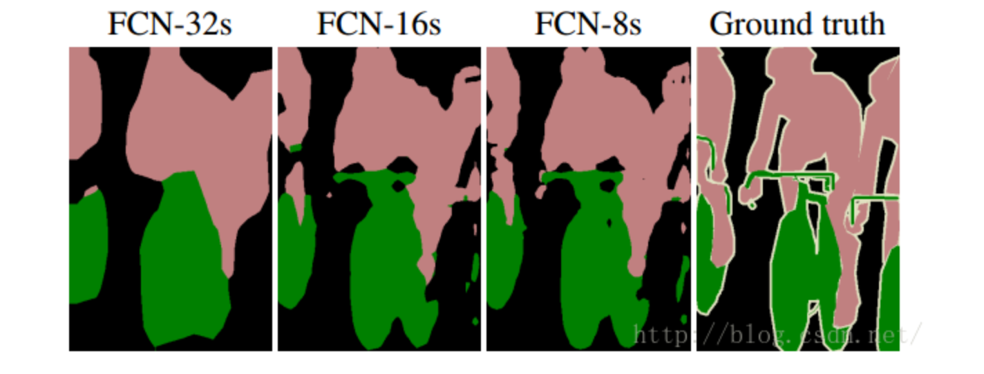
作者认为CNN网络输出的结果偏向与smooth(如何smooth可以见下图),因此对DeepMedic网络(11层,dual pathways)网络的输出认为是soft segmentation。最后作者用CRF对soft segmentations 进行后处理(post-processing)改善其边缘信息。
5.1 为什么CRF可以用于处理图像任务?
首先对于图像任务,我们可以把每个像素认为是一个单独的节点(node),像素与像素之间就构成了边(edge),同时,相邻像素之间相互影响,而这种影响是对称的,相当于edge,因此构成了一个概率无向图。
5.2 全连接条件随机场
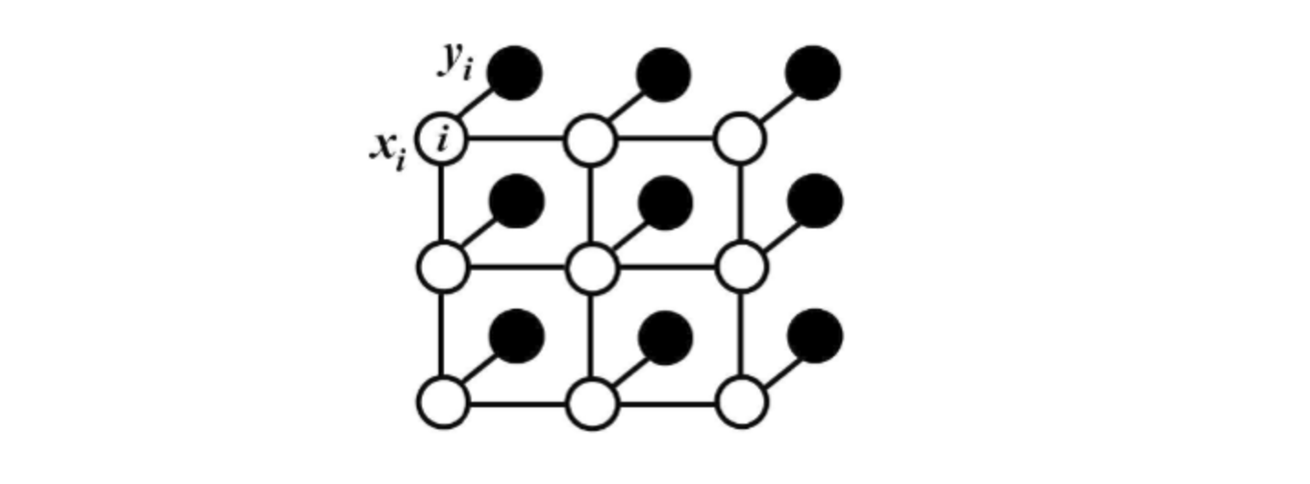
对于每个像素 $i$ 具有类别标签 $x_i$ 还有对应的观测值 $y_i$,这样每个像素点作为节点,像素与像素间的关系作为边,即构成了一个条件随机场。而且我们通过观测变量 $y_i$ 来推测像素 $i$ 对应的类别标签 $x_i$。条件随机场如下:
条件随机场符合吉布斯分布:(此处的 $x$ 即上面说的观测值)
$$P(\boldsymbol{X} = \mathbf{x} | \boldsymbol{I}) = \frac{1}{Z(\boldsymbol{I})} exp\left( -\mathbb{E}(\mathbf{x}|\boldsymbol{I}) \right) $$
其中的 $\mathbb{E}(\mathbf{x}|\boldsymbol{I})$ 是能量函数,为了简便,以下省略全局观测 $\boldsymbol{I}$:
$$ E(\mathbf{x})=\sum_i{\Psi_u(x_i)}+\sum_{i,j}\Psi_p(x_i, x_j) $$其中的一元势函数 $\sum_i{\Psi_u(x_i)}$ 即来自于前端FCN的输出。而二元势函数如下:
$$\Psi_p(x_i, x_j)=u(x_i, x_j)\sum_{m=1}^M{\omega^{(m)}k_G^{(m)}(\boldsymbol{f_i, f_j)}}$$二元势函数就是描述像素点与像素点之间的关系,鼓励相似像素分配相同的标签,而相差较大的像素分配不同标签,而这个“距离”的定义与颜色值和实际相对距离有关。所以这样CRF能够使图片尽量在边界处分割。
而全连接条件随机场的不同就在于,二元势函数描述的是每一个像素与其他所有像素的关系,所以叫“全连接”。
Reference
Harvard Referencing: Kamnitsas, K., Ledig, C., Newcombe, V.F., Simpson, J.P., Kane, A.D., Menon, D.K., Rueckert, D. and Glocker, B., 2017. Efficient multi-scale 3D CNN with fully connected CRF for accurate brain lesion segmentation. Medical image analysis, 36, pp.61-78.
- Title: DeepMedic - multi-sacle 3D CNN with CRF for brain lesion segmentation
- Author: Zhanhang (Matthew) ZENG
- Link: https://zengzhanhang.com/2019/07/18/deepmedic/
- Released Date: 2019-07-18
- Last update: 2020-05-21
- Statement: All articles in this blog, unless otherwise stated, are based on the CC BY-NC-SA 4.0 license.